Slicing Skulls and Counting Triangles: A Volumetric Rendering Pipeline in C++ and Vulkan
Introduction
Medical imaging is one of the rare domains where you can hold a 3D array of numbers in memory and reasonably call it a person. A CT volume is a stack of 2D slices, each one a thin cross-section captured at a different depth. The engineering question is what to do with it: how do you turn millions of voxels into something a clinician can see, navigate, and trust?
This project was a build-from-scratch volumetric viewer in C++ with Vulkan, working with a real CT dataset of a human skull. It covered three pieces of the pipeline: arbitrary 2D reslicing, surface extraction via marching cubes, and a real-time shader path with fly-through navigation. Each part had its own surprise — usually about how much the geometry of the data dictates what you can do with it.
Reslicing anisotropic data
CT scanners capture data in stacks of axial slices. The within-slice resolution (0.05 cm per pixel) is much finer than the inter-slice spacing (Δz ≈ 2.44 voxel units, about 50× coarser). This is anisotropic data, and it matters the moment you try to view it from any angle the scanner didn’t natively capture.
The first task was nearest-neighbour reslicing in the XZ and YZ planes. The naïve approach maps each pixel of the reslice image to the nearest stored voxel:
for (z = 0; z < VOLUME_DEPTH; z++) {
    nearest_slice = round(z / DELTA_Z);
    data_index = nearest_slice * VOLUME_WIDTH * VOLUME_HEIGHT
               + (int)round(y_reslice_position) * VOLUME_WIDTH;

    for (x = 0; x < VOLUME_WIDTH; x++) {
        texture_store.xz_rgba[reslice_index++] = MapItoR[data[data_index]];
        // ...G, B, A
        data_index++;
    }
}
This works, but the result has prominent horizontal banding:
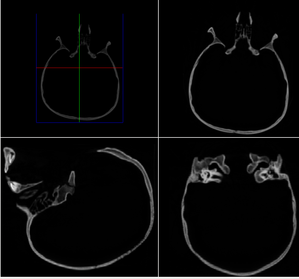
The cause is direct: with Δz ≈ 2.44, each acquired slice gets “held” for roughly 2–3 rows in the reslice image before the index jumps to the next slice. The staircase pattern is most visible in soft-tissue regions where intensity changes gradually.
Switching to linear interpolation — blending the two bracketing slices in proportion to fractional z-distance — eliminates the banding:
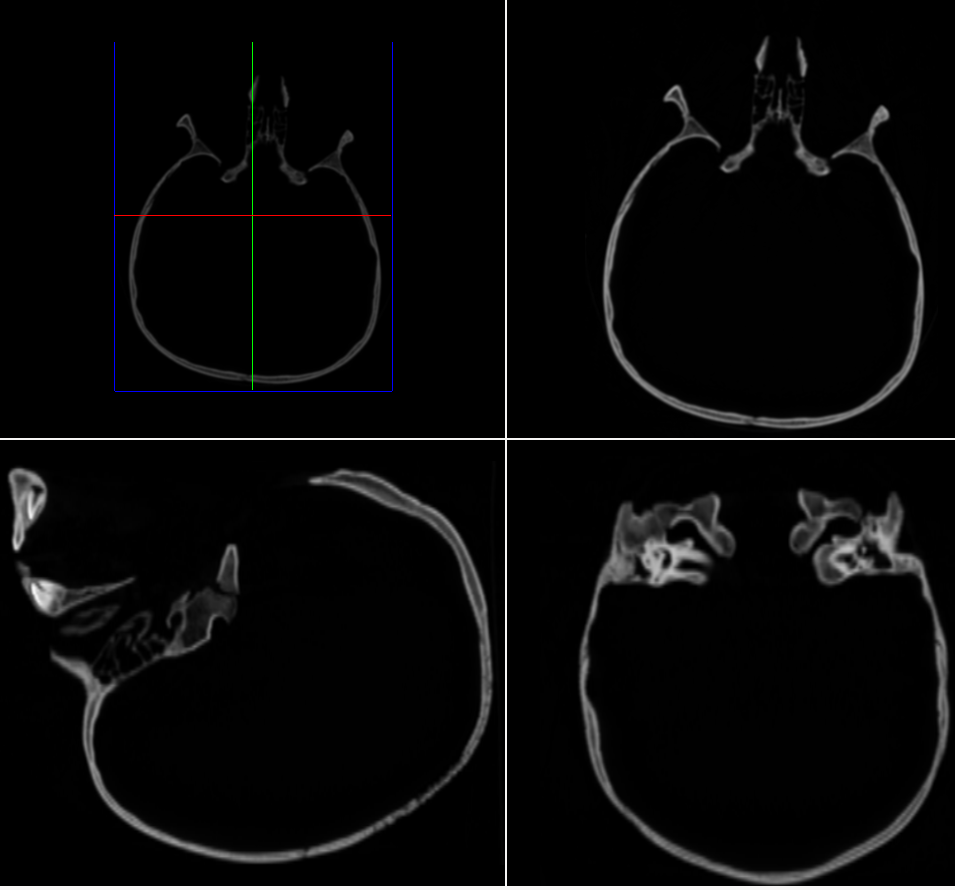
The trade-off is mild blurring of sharp boundaries: cortical bone edges appear slightly wider because interpolation blends surrounding tissue into them. For diagnostic viewing this is almost always the right trade — banding looks like an artefact, blur looks like resolution.
The lesson here was more general: the aspect ratio of your data isn’t just a display concern. A 50:1 axis ratio doesn’t mean the data is “stretched” — it means certain views cannot be reconstructed faithfully without interpolation. Anisotropy is a property of the sampling, not the rendering.
Marching cubes and the geometry of “inside”
The next task was surface extraction: given a 3D scalar field, produce a triangle mesh of the isosurface at some threshold. The marching cubes algorithm steps through the volume cube-by-cube, classifies each of the 8 corner voxels as inside or outside, and looks up a triangulation in a 256-entry table.
It has two knobs: the threshold (what counts as inside?) and the resolution (how big are the cubes?). The interesting part is how unintuitively they interact. Lower threshold = more voxels classified as inside, so larger enclosed volume. Fine. But lowering the threshold on CT data also reduces the triangle count:
| Threshold | Resolution | #Triangles | Volume (ml) |
|---|---|---|---|
| 30 (bone) | 4 | 86,760 | 551.0 |
| 30 (bone) | 1 | 1,189,162 | 567.5 |
| 10 (+soft tissue) | 4 | 75,782 | 686.6 |
| 10 (+soft tissue) | 1 | 1,147,802 | 692.9 |
Intuitively, more volume should mean more surface. It doesn’t, because the shape changes. At threshold 30 you isolate cortical bone, which has a trabecular, highly irregular surface — lots of triangles per unit volume. At threshold 10 you envelop the bone in a smoother soft-tissue boundary that contains more enclosed space with less surface area. Geometry wins over volume.
The resolution parameter is more predictable. Doubling the cube edge length divides the cell count by 8, so triangle count drops roughly by a factor of 8. The enclosed volume also converges as resolution increases — a useful sanity check: if your reported volume swings wildly between resolutions, something is wrong with the implementation, not the data.
A note on memory
There are two ways to store a triangle mesh. The complete form stores three full vertex records per triangle (72 bytes each). The indexed form stores the vertex array once and triangles as triples of indices, costing about 48 bytes per vertex.
For a closed mesh, Euler’s formula gives T ≈ 2V, so M_complete ≈ 144V vs M_indexed ≈ 48V — a clean 3× saving from sharing. On the 42,868-vertex skull mesh, that’s 6.1 MB vs 2.0 MB. Nothing exotic, but a good reminder that data structure choices compound: every triangle shares vertices with neighbours, and pretending otherwise wastes most of your memory.
Shaders and the cost of pretty highlights
The final part was the rendering pipeline. The viewer supports two shading models: Gouraud (per-vertex lighting, interpolated across the triangle) and Phong (per-fragment lighting, evaluated for every pixel). Phong gives noticeably better specular highlights — Gouraud’s interpolation can make highlights pop on and off as you rotate. But Phong does more work, and at high triangle counts the cost shows up in the frame rate:
| Shader | Avg fps |
|---|---|
| Phong | 5,100 |
| Gouraud | 6,250 |
A ~20% hit for Phong on this dataset. The interesting thing is where the cost lives. Phong is fragment-shader-bound: the full Blinn-Phong equation (including pow() for the specular term) runs once per pixel. Gouraud is vertex-bound: the same calculation runs once per vertex, with cheap linear interpolation across each triangle. When the surface has many more pixels than vertices on screen — the common case for foreground geometry — Gouraud wins easily.
Some quick measurements made the bottleneck structure visible:
- Close to the surface (lots of fragments): ~4,200 fps
- Far from the surface (few fragments): ~6,680 fps
- Surface outside view frustum (zero fragments, vertices still processed): ~6,700 fps
- Surface drawing disabled entirely (no GPU work at all): ~14,800 fps
The numbers tell a clean story. Going from close-up to far away recovers ~2,500 fps — that’s the fragment shader workload. Going from far away to outside-frustum recovers nothing — culling already eliminated the fragment work but kept the vertex shader running. Going from outside-frustum to not-drawing-at-all recovers another 8,000 fps — that’s the vertex pipeline cost itself.
That breakdown isn’t an interpretation of the numbers; it’s effectively a profiling pass disguised as a fly-through. Each stage of the GPU pipeline is observable just by changing what’s on screen.
Reflections
A few takeaways I’ll keep.
Data shape dictates what views are possible. Anisotropic CT data isn’t a Cartesian volume you happen to view from a Cartesian angle — its sampling is the dominant fact about it. Interpolation isn’t a smoothing technique here; it’s a reconstruction technique, the only way to recover directions the scanner didn’t capture.
Triangle count is decoupled from geometric size. The lower-threshold case had more enclosed volume and fewer triangles, because soft tissue is smoother than bone. This is one of those results that rewires your intuition: the cost of representing a surface depends on its roughness, not on how much it contains.
The graphics pipeline is observable, not just abstract. Watching the frame rate triple as the surface left the frustum made “vertex shader” and “fragment shader” feel like real, measurable workloads rather than boxes in a diagram. You can profile the pipeline by moving the camera.